Probabilistic Forecasting (Supply Chain)

By Joannes Vermorel, November 2020

A forecast is said to be probabilistic, instead of deterministic, if it contains a set of probabilities associated with all possible future outcomes, instead of pinpointing one particular outcome as “the” forecast. Probabilistic forecasts are important whenever uncertainty is irreducible, which is nearly always the case whenever complex systems are concerned. For supply chains, probabilistic forecasts are essential to produce robust decisions against uncertain future conditions. In particular, demand and lead time, two key aspects of the supply chain analysis, are both best addressed via probabilistic forecasting. The probabilistic perspective lends itself naturally to the economic prioritization of the decisions based on their expected but uncertain returns. A large variety of statistical models deliver probabilistic forecasts. Some are structurally close to their deterministic counterparts while others are very different. Assessing the accuracy of a probabilistic forecast requires specific metrics, which differ from their deterministic counterparts. The exploitation of probabilistic forecasts requires specialized tooling that diverges from its deterministic counterparts.

Deterministic vs. Probabilistic forecasts    Supply chain use cases       In defense of variability    The Law of Small Numbers    Accuracy metrics for probabilistic forecasts       Vanishingly small probabilities and log likelihood    Algorithmic flavors of probabilistic forecasts    Working with probabilistic forecasts    Visualization of probabilistic forecasts    Probabilistic forecasting antipatterns       No such thing as ‘unpredictable’ events       No such thing as ‘normal’ distributions       Cherry-picking probabilities       Removing statistical outliers       Bringing a sword to a gunfight    Notes

Deterministic vs. Probabilistic forecasts

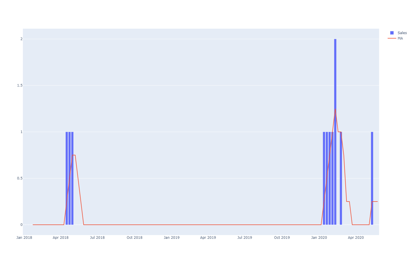
The optimization of supply chains relies on the proper anticipation of future events. Numerically, these events are anticipated through forecasts, which encompass a large variety of numerical methods used to quantify these future events. From the 1970s onward, the most widely used form of forecast has been the deterministic time-series forecast: a quantity measured over time - for example the demand in units for a product - is projected into the future. The past section of the time-series is the historical data, the future section of the time-series is the forecast.


MA stands for "moving average", it's not particularly well-behaved on sparse time-series.

These time-series forecasts are said to be deterministic because for every point of time in the future, the forecast provides a single value that is expected to match the future outcome as closely as possible. Indeed, while the forecast is single valued, it is widely understood that the forecast has little chance to be perfectly correct. Future outcomes will diverge from the forecast. The adherence of the deterministic forecast to its future outcomes is quantitatively assessed through accuracy metrics, such as the mean square error (MSE) for example.

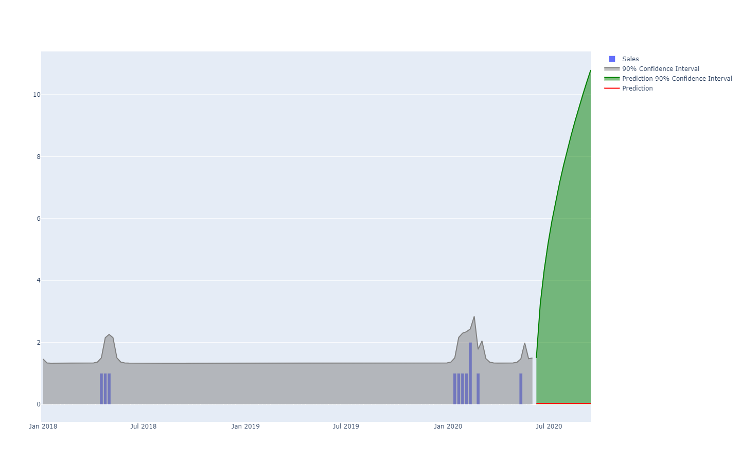
Probabilistic forecasts adopt a different perspective on the anticipation of future outcomes. Instead of producing one value as the “best” outcome, the probabilistic forecast consists of assigning a probability to every possible outcome. In other words, all future events remain possible, they are just not equally probable. Below is the visualization of a probabilistic time-series forecast exhibiting the “shotgun effect”, which is typically observed in most real-world situations. We will be revisiting this visualization in greater details in the following.


A probabilistic forecast illustrating a high-uncertainty situation.

Time-series, a quantity measured over time, is probably the most widely-known and most widely-used data model. This data model can be forecast both through deterministic or probabilistic means. However, there are many alternative, typically richer, data models that also lend themselves to forecasts of both kinds. For example, a company that repairs jet engines may wish to anticipate the exact list of spare parts that will be needed for an upcoming maintenance operation. This anticipation can take the form of a forecast, but it won’t be a time-series forecast. The deterministic forecast associated with this operation is the exact list of parts and their quantities. Conversely, the probabilistic forecast is the probability for every combination of parts (quantities included) that this specific combination will be the one needed to perform the repairs.

Also, while the term “forecast” emphasizes an anticipation of some kind, the idea can be generalized to any kind of statistically inferred statement about a system, including for its past (but unknown) properties. The statistical forecasting practice emerged during the 20th century, before the advent of the more modern statistical learning perspective, which encompasses all the data-driven extrapolations that can be performed, irrespective of any temporal dimension. For the sake of clarity, we will keep using the term “forecast” in the following, even if the temporal aspect does always equate past with known and future with unknown. For example, a company may wish to estimate the sales that would have taken place for a product in a store if the product had not been out-of-stock this day. The estimation is useful to quantify the magnitude of the problem in terms of quality of service. However, as the event is past, the “real” sales figure will never be observed. Nevertheless, assuming it has not yet been trivially observed, the statistical estimation of the past demand is a problem that is very close to the estimation of the future demand.

Probabilistic forecasts are richer - information-wise - than their deterministic counterparts. While the deterministic forecast provides a “best guess” of the future outcome, it says nothing about the alternatives. In fact, it is always possible to convert a probabilistic forecast into its deterministic counterpart by taking the mean, the median, the mode, ... of the probability distribution. Yet, the opposite does not hold true: it is not possible to recover a probabilistic forecast from a deterministic one.

Yet, while probabilistic forecasts are statistically superior to deterministic forecasts, they remain infrequently used in supply chain. However, their popularity has been steadily increasing over the last decade. Historically, probabilistic forecasts emerged later, as they require significantly more computing resources. Leveraging probabilistic forecasts for supply chain purposes also requires specialized software tools, which are also frequently unavailable.

Supply chain use cases

Optimizing a supply chain consists of taking the “right” decision - at the present point of time - which will most profitably address a future situation that is only imperfectly estimated. However, the uncertainty associated with future events is irreducible to a large extent. Thus, the company needs the decision to be robust if the anticipation of the future event - i.e. the forecast - is imperfect. This has been done minimally since the mid 20th century through the safety stock analysis. However, as we will see below, beside historical interest, there is no longer any reason to favor safety stocks over “native” probabilistic numerical recipes.

The probabilistic forecasting perspective takes a radical stance towards uncertainty: this approach attempts to quantify the uncertainty to the greatest extent. In supply chain, costs tend to be concentrated on the statistical extremes: it’s the unexpectedly high demand that creates the stockout, it’s the unexpectedly low demand that creates the inventory write-off. In between, the inventory rotates just fine. Probabilistic forecasts are - crudely put - an attempt at managing these low-frequency, high-cost situations that are ubiquitous in modern supply chains. Probabilistic forecasts can and should be seen as a core ingredient of any risk management practice within the supply chain.

Many aspects of supply chains are particularly suitable for probabilistic forecasting, such as:

• demand: garments, accessories, spare parts; as well as many other types of products, tend to be associated with erratic and/or intermittent demand. Product launches may be hit or miss. Promotions from competitors may temporarily and erratically cannibalize large portions of the market shares.
• lead time: oversea imports can incur a whole series of delays at any point of the chain (production, transport, customs, reception, etc). Even local suppliers may infrequently have long lead times if they face a stock-out problem. Lead times tend to be “fat tailed” distributions.
• yield (fresh food): the quantity and the quality of the production of many fresh products depend on conditions, such as the weather, which are outside the company’s control. The probabilistic forecast quantifies these factors for the entire season and offers the possibility to go beyond the horizon of relevance of classic weather forecasts.
• returns (ecommerce): when a customer orders the same product in three different sizes, the odds are high that two of those sizes will be returned. More generally, while strong regional differences exist, customers tend to leverage favorable return policies when those exist. The probability of returns for each order should be assessed.
• scraps (aviation): repairable aircraft parts - frequently referred to as rotables - sometimes fail to be repaired. In this case, the part is scrapped, as it is unsuitable to ever be mounted again on an aircraft. While it is usually not possible to know in advance whether a part will survive its repair or not, the odds of having the part scrapped should be estimated.
• stocks (B2C retail): customers may displace, damage or even steal goods from a retail store. Thus, the electronic stock level is only an approximation of the real on-shelf availability as perceived by customers. The stock level, as perceived by customers, should be estimated through a probabilistic forecast.
• …
  

This short list illustrates that the angles eligible for a probabilistic forecast vastly exceed the sole traditional, “demand forecasting” angles. The well-engineered optimization of a supply chain requires to factor all the relevant sources of uncertainty. While it is sometimes possible to reduce the uncertainty - as emphasized by lean manufacturing - there are usually economic trade-offs involved, and as a result, some amount of uncertainty remains irreducible.

Forecasts, however, are merely educated opinions about the future. While probabilistic forecasts may be considered as remarkably fine-grained opinions, they are not fundamentally different from their deterministic counterparts in this regard. The value, supply chain wise, of the probabilistic forecasts is found in the way that this fine structure is exploited to deliver more profitable decisions. In particular, probabilistic forecasts are typically not expected to be more accurate than their deterministic counterparts if deterministic accuracy metrics are used to assess the quality of the forecasts.

In defense of variability

Despite what many approaches to supply chain advocate, variability is here to stay - hence the need for probabilistic forecasts. The first misconception is that variability is necessarily a bad thing for a supply chain; it isn’t. The second misconception is that variability can be engineered away; it can’t.

Variability has positive implications for supply chains in multiple situations. For example, on the demand side, most verticals are driven by novelty, such as fashion, cultural products, soft and hard luxury - as are “hit or miss” businesses. Most new products aren’t successes (misses), but the ones that succeed (hits) yield massive returns. Extra variability is good because it increases the probability of outsized returns, while downsides remain capped (worst case, the whole inventory is written off). The neverending stream of new products pushed to market ensures the constant renewal of “hits”, while the old ones are waning.

On the supply side, a sourcing process that ensures highly variable pricing offers is superior - all things considered equal - to an alternative process that generates much more consistent (i.e. less variable) prices. Indeed, the lowest priced option is selected while the others are dismissed. It does not matter whether the “average” sourced price is low, what matters is uncovering lower priced sources. Thus, the good sourcing process should be engineered to increase variability, for example by emphasizing the routine exploration of new suppliers as opposed to restricting the sourcing process to the well-established ones.

Sometimes, variability may be beneficial for more subtle reasons. For example, if a brand is too predictable when it comes to its promotional operations, customers identify the pattern and start delaying their purchase as they know that a promotion is coming and when. Variability - erraticity even - of the promotional activities mitigates this behavior to some extent.

Another example is the presence of confusion factors within the supply chain itself. If new products are always launched with both a TV campaign and a radio campaign, it becomes statistically difficult to distinguish the respective impacts of the TV and of the radio. Adding variability to the respective campaign intensity depending on the channel ensures that more statistical information can be extracted from those operations afterward, which can be later on turned into insights for a better allocation of the marketing resources.

Naturally, all variability isn’t good. Lean manufacturing is correct to emphasize that, on the production side of the supply chain, variability is usually detrimental, especially when it comes to varying delays. Indeed, LIFO (last-in first-out) processes may accidentally creep in, which, in turn, exacerbates lead time variability. In those situations, the accidental variability should be engineered away, typically through a better process, sometimes through better equipment or facilities.

Variability - even when detrimental - is frequently irreducible. As we will see in the following section, supply chains abide to the law of small numbers. It is delusional to think that store-level will ever be reliably predicted - from a deterministic perspective - while customers don’t always know themselves what they are about to buy. More generally, reducing variability always comes at a cost (and lowering it further costs even more), while the marginal reduction of variability only brings diminishing returns. Thus, even when variability can be reduced, for all intents and purposes, it can very rarely be entirely eliminated due to the economic implications.

The Law of Small Numbers

The supply chain law of small numbers can be stated as: small numbers prevail everywhere along the chain. This observational law results from the economies of scale and a few other forces that drive most of the structural aspects of supply chains:

• a supplier that provides tens of thousands of units of materials per day is likely to have minimal order quantities (MOQ) or price breaks that prevent purchase orders to be made too frequently. The number of purchase orders passed on any given day to a supplier rarely exceeds a single digit number.
• a factory that produces tens of thousands of units per day is likely to operate through large batches of thousands of units. The production output is likely to be packaged through entire pallets. The number of batches during any given day is at most a small, two digit number.
• a warehouse that receives tens of thousands of units per day is likely to be delivered by trucks, each truck unloading its entire cargo into the warehouse. The number of truck deliveries any given day rarely exceeds a two-digit number, even for very large warehouses.
• a retail store that can hold tens of thousands of units in stock is likely to spread its assortment in thousands of distinct product references. The number of units held in stock for each product very rarely exceeds a single digit number.
• ...
  

Naturally, by changing the unit of measurement, it is always possible to inflate the numbers. For example, if instead of counting the number of pallets we count the number of grams of pallets, or their monetary values in USD cents, large numbers appear. However, the law of small numbers should be understood with the notion of counting things from a sensible supply chain perspective. While, in theory, this principle may appear fairly subjective, it is not the case in practice, due to the obvious discrete practicalities of modern supply chains: bundles, boxes, pallets, containers, trucks …

This law is of high relevance for the probabilistic forecasting perspective. First, it outlines that discrete forecasts dominate in supply chain situations, i.e. the outcome to be anticipated (or decided) is an integer , as opposed to a fractional number. Probabilistic forecasts are particularly suitable for discrete situations, because a probability can be estimated for each discrete outcome. In contrast, deterministic forecasts struggle with discrete outcomes. For example, what is it supposed to mean that the expected daily sales of a product are at 1.3 units? Units aren’t sold fractionally. While more sensical “discrete” interpretations can be inferred from this statement, its probabilistic counterpart (e.g. 27% chance of 0 unit of demand, 35% chance of 1 unit of demand, 23% chance of 2 units of demand, etc.) is much more straightforward, because it embraces the discrete nature of the phenomenon of interest.

Second, while probabilistic forecasts may appear to be radically more challenging in terms of raw computing resources, this is not really the case in practice, precisely due to the law of small numbers. Indeed, going back to the daily product sales discussed above, there is no point in numerically assessing the odds where the demand is going to exceed 100 on any given day. Those probabilities can be rounded to zero - or some arbitrary vanishingly small value. The impact on the numerical accuracy of the supply chain model remains negligible. As a rule of thumb, it’s reasonable to consider that probabilistic forecasts require about three orders of magnitude more computing resources than their deterministic counterparts. However, despite this overhead, the benefits in terms of supply chain performance vastly exceed the cost of the computing resources.

Accuracy metrics for probabilistic forecasts

No matter what happens, a reasonably well-designed probabilistic forecast indicates that there was indeed a non-zero probability for this outcome to happen. This is intriguing because at a first glance, it may appear as if probabilistic forecasts were somehow immune to the reality, just like a fortune teller making vastly ambiguous prophetic statements that can’t ever be proven wrong, as the fortune teller can always conjure a later explanation about the proper way to interpret the prophecies after the fact. In reality, there exist multiple ways to quantitatively assess the quality of a probabilistic forecast. Some of these ways are metrics similar in spirit to the metrics used to assess the accuracy of deterministic forecasts. Some other ways diverge into more radical and more profound ways compared to the deterministic perspective.

Let’s briefly review four distinct approaches to assess the accuracy of a probabilistic forecast:

• the pinball loss function
• the continuous ranked probability score (CRPS)
• the Bayesian likelihood
• the generative adversarial perspective
  

The pinball loss function provides an accuracy metric for a quantile estimate to be derived from a probabilistic forecast. For example, if we wish to assess the stock quantity that has 98% chance to be greater or equal to the customer demand in a store for a given product, this quantity can be obtained directly from the probabilistic forecasts by merely summing the probabilities starting from 0 unit of demand, 1 unit of demand, … until the probability just exceeds 98%. The pinball loss function provides a direct measurement of the quality of this biased estimate of the future demand. It can be seen as a tool to assess the quality of any point of the probabilistic forecast’s cumulative density function.

The continuously ranked probability score (CRPS) provides a metric, which can be interpreted as the “amount of displacement” of the mass of probabilities that it takes to move all the probability mass to the observed outcome. It is the most direct generalization of the mean absolute error (MAE) toward a probabilistic perspective. The CRPS value is homogeneous with the unit of measurement of the outcome itself. This perspective can be generalized to arbitrary metric spaces, instead of just one-dimensional situations, through what is known as the “transportation theory” and Monge-Kantorovich distance (which goes beyond the scope of the present document).

The likelihood and its cross-entropy cousin adopts the Bayesian perspective of the least degree of surprise: the higher the probability of the observed outcomes, the better. For example, we have two probabilistic models A and B: the model A states that the probability of observing 0 unit of demand is 50% for any given day; the model B states that the probability of observing 0 unit of demand is 1% for any given day. We observe the demand over 3 days and get the following observations: 0, 0, 1. The model A had roughly a 10% chance of generating these observations, while for the model B, it was only a rough 0.01% chance. Thus, the model B is vastly less likely to be the correct model compared to model A. The likelihood diverges from the deterministic perspective of having a meaningful absolute criterion to assess models. Instead, it provides a mechanism to compare models, but numerically, the mechanism can’t really be used for anything but comparing models.

The generative adversarial perspective is the most modern perspective on the matter (Ian Goodfellow et al., 2014). Essentially, this perspective states that the “best” probabilistic model is the one that can be used to generate outcomes - monte-carlo style - that are indistinguishable from real outcomes. For example, if we were to consider the historical list of transactions at a local hypermarket, we could truncate this history at an arbitrary point of time in the past and use the probabilistic model to generate fake but realistic transactions onward. The model would be deemed as “perfect” if it was impossible, through statistical analysis, to recover the point of time where the dataset transitions from “real” to “fake” data. The point of the generative adversarial approach is to “learn” the metrics that exacerbate the flaw of any probabilistic model. Instead of focusing on a particular metric, this perspective recursively leverages machine learning techniques to “learn” the metrics themselves.

Seeking better ways to access the quality of probabilistic forecasts is still an active area of research. There is no clear delimitation between the two questions “How to produce a better forecast?” and “How to tell if a forecast is better?”. Recent works have considerably blurred the lines between the two, and it’s likely that the next breakthroughs will involve further shifts in the very way probabilistic forecasts are even looked at.

Vanishingly small probabilities and log likelihood

Very small probabilities naturally arise when looking at a many-dimensional situation through the prism of probabilistic forecasts. Those small probabilities are troublesome because computers are not processing indefinitely precise numbers. Raw probability values are frequently “vanishingly” small in the sense that they get rounded to zero due to limits on numerical precision. The solution to this problem is not to upgrade the software toward arbitrary-precision calculations - which is very inefficient in terms of computing resources - but to use the “log-trick”, which transforms multiplications into additions. This trick is leveraged - one way or another - by virtually every piece of software dealing with probabilistic forecasts.

Let’s assume that we have $X_1$, $X_2$, …, $X_n$ random variables representing the demand of the day for all the $n$ distinct products served within a given store. Let $\hat{x}_1$, $\hat{x}_2$, .., $\hat{x}_n$ correspond to the empirical demand observed at the end of the day for each product. For the first product - governed by $X_1$ - the probability of observing $\hat{x}_1$ is written $P(X_1 = \hat{x}_1)$. Now, let’s assume, somewhat abusively but for the sake of clarity, that all products are strictly independent demand-wise. The probability for the joint event of observing $\hat{x}_1$, $\hat{x}_2$, .., $\hat{x}_n$ is:

$$P(X_1 = \hat{x}_1 \dots X_n = \hat{x}_n) = \prod_{k=1}^n P(X_k = \hat{x}_k)$$ If $P(X_k = \hat{x}_k) \approx \frac{1}{2}$ (gross approximation) and $n = 10000$ then the joint probability above is of the order $\frac{1}{2^{10000}} \approx 5 * 10^{-3011}$, which is a very small value. This value underflows, i.e. goes below the small representable number, even considering 64-bit floating point numbers which are typically used for scientific computing.

The “log-trick” consists of working with the logarithm of the expression, that is:

$$\ln P(X_1 = \hat{x}_1 \dots X_n = \hat{x}_n) = \sum_{k=1}^n \ln P(X_k = \hat{x}_k)$$ The logarithm turns the series of multiplications into a series of additions, which proves to be much more numerically stable than a series of multiplications.

The usage of the “log-trick” is frequent whenever probabilistic forecasts are involved. The log likelyhood is quite literally the logarithm of the likelihood (introduced previously) precisely because the raw likelihood would usually be numerically un-representable considering the common types of floating point numbers.

Algorithmic flavors of probabilistic forecasts

The question of the computer-driven generation of probabilistic forecasts is almost as vast as the field of machine learning itself. The delimitations between the two fields, if any, are mostly a matter of subjective choices. Nevertheless, this section presents a rather elective list of notable algorithmic approaches that can be used to obtain probabilistic forecasts.

In the early 20th century, possibly in the late 19th century, the idea of the safety stock emerged, where the demand uncertainty is modeled after a normal distribution. As pre-computed tables of the normal distribution had already been established for other sciences, notably physics, the application of safety stock only required a multiplication of a demand level by a “safety stock” coefficient pulled from a pre-existing table. Anecdotally, many supply chain textbooks written until the 1990s still contained tables of the normal distribution in their appendices. Unfortunately, the main drawback of this approach is that normal distributions are not a reasonable proposition for supply chains. First, as far as supply chains are concerned, it’s safe to assume that nothing is ever normally distributed. Second, the normal distribution is a continuous distribution, which is at odds with the discrete nature of supply chain events (see “Law of small numbers” above). Thus, while technically “safety stocks” have a probabilistic component, the underlying methodology and numerical recipes are resolutely geared toward the deterministic perspective. This approach is listed here however for the sake of clarity.

Fast forward to the early 2000s, ensemble learning methods - whose most well-known representatives are probably random forests and gradient boosted trees - are relatively straightforward to extend from their deterministic origins to the probabilistic perspective. The key idea behind ensemble learning is to combine numerous, weak, deterministic predictors, such as decision trees, into a superior deterministic predictor. However, it is possible to adjust the mixing process to obtain probabilities rather than just a single aggregate, hence turning the ensemble learning method into a probabilistic forecasting method. These methods are non-parametric and capable of fitting fat-tailed and/or multimodal distributions, as commonly found in the supply chain. These methods tend to have two notable downsides. First, by construction, the density probability function produced by this class of models tends to include a lot of zeroes, which prevents any attempts at leveraging the log-likelihood metric. More generally, these models don’t really fit the Bayesian perspective, as newer observations are frequently declared “impossible” (i.e. zero probability) by the model. This problem however can be solved through regularization methods[1]. Second, models tend to be as large as a sizable fraction of the input dataset, and the “predict” operation tends to be almost as computationally costly as the “learn” operation.

The hyper-parametric methods collectively known under the name of “deep learning”, which explosively emerged in the 2010s were, almost accidentally, probabilistic. Indeed, while the vast majority of the tasks where deep learning really shines (e.g. image classification) only focus on deterministic forecasts, it turns out that the cross-entropy metric - a variant of the log likelihood discussed above - exhibits very steep gradients that are frequently well suited for the stochastic gradient descent (SGD), which lies at the deep learning methods’ core. Thus, the deep learning models turn out to be engineered as probabilistic, not because probabilities were of interest, but because the gradient descent converges faster when the loss function reflects a probabilistic forecast. Thus, with regards to deep learning, supply chain distinguishes itself by its interest for the actual probabilistic output of the deep learning model, while most other use cases are collapsing the probability distribution to its mean, median or mode. The Mixture Density Networks is a type of deep learning network geared toward learning complex probability distributions. The result itself is a parametric distribution, possibly made of Gaussians. However, unlike ‘safety stocks, a mixture of many Gaussian may, in practice, reflect the fat-tail behaviors that are observed in the supply chains. While deep learning methods are frequently considered as state-of-art, it must be noted that achieving numerical stability, especially when density mixtures are involved, remains a bit of a “dark art”.

Differentiable programming is a descendent of deep learning, which gained popularity in the very late 2010s. It shares many technical attributes with deep learning, but differs significantly in focus. While deep learning focuses on learning arbitrary complex functions (i.e. playing Go) by stacking a large number of simple functions (i.e. convolutional layers), differentiable programming focuses on the learning process’ fine-structure. The most fine-grained, most expressive structure, quite literally, can be formatted as a program, which involves branches, loops, function calls, etc. Differentiable programming is of high interest for the supply chain, because problems tend to present themselves in ways that are highly structured, and those structures are known to the experts[2]. For example, the sales of a given shirt can be cannibalized by another shirt of a different color, but it won’t be cannibalized by the sales of a shirt three sizes apart. Such structural priors are key to achieve high data efficiency. Indeed, from a supply chain perspective the amount of data tends to be very limited (cf. the law of small numbers). Hence, structurally “framing” the problem helps to ensure that the desired statistical patterns are learned, even when facing limited data. Structural priors also help to address numerical stability problems as well. Compared to ensemble methods, structural priors tend to be a less time-consuming affair than feature engineering; model maintenance is also simplified. On the downside, differentiable programming remains a fairly nascent perspective to date.

The Monte Carlo perspective (1930 / 1940) can be used to approach probabilistic forecasts from a different angle. The models discussed so far are providing explicit probability density functions (PDFs). However, from a Monte Carlo perspective, a model can be replaced by a generator - or sampler - which randomly generates possible outcomes (sometimes called “deviates”). PDFs can be recovered by averaging the generator’s results, although PDFs are frequently bypassed entirely in order to reduce the requirements in terms of computational resources. Indeed, the generator is frequently engineered to be vastly more compact - data-wise - than the PDFs it represents. Most of the machine learning methods - including those listed above to directly tackle probabilistic forecasts - can contribute to learning a generator. Generators can take the form of low-dimensional parametric models (e.g. state space models) or of hyper-parametric models (e.g. the LSTM and GRU models in deep learning). Ensemble methods are rarely used to support generative processes due to their high compute costs for their “predict” operations, which are extensively relied upon to support the Monte Carlo approach.

Working with probabilistic forecasts

Deriving useful insights and decisions from probabilistic forecasts requires specialized numerical tooling. Unlike deterministic forecasts where there are plain numbers, the forecasts themselves are either explicit, probability density functions, or Monte Carlo generators. The quality of the probabilistic tooling is, in practice, as important as the quality of the probabilistic forecasts. Without this tooling, the exploitation of the probabilistic forecasts devolves into a deterministic process (more on this in the “Antipatterns” section below).

For example, the tooling should be able to perform tasks such as:

• Combine the uncertain production lead time with the uncertain transport lead time, to get the “total” uncertain lead time.
• Combine the uncertain demand with the uncertain lead time, to get the “total” uncertain demand to be covered by the stock about to be ordered.
• Combine the uncertain order returns (ecommerce) with the uncertain arrival date of the supplier order in transit, to get the uncertain customer lead time.
• Augment the demand forecast, produced by a statistical method, with a tail risk manually derived from a high-level understanding of a context not reflected by the historical data, such as a pandemic.
• Combine the uncertain demand with an uncertain state of the stock with regards to the expiration date (food retail), to get the uncertain end-of-day stock leftover.
• ...
  

Once all probabilistic forecasts - not just the demand ones - are properly combined, the optimization of the supply chain decisions should take place. This involves a probabilistic perspective on the constraints, as well as the score function. However, this tooling aspect goes beyond the scope of the present document.

There are two broad “flavors” of tools to work with probabilistic forecasts: first, algebras over random variables, second, probabilistic programming. These two flavors supplement each other as they don’t have the same mix of pros and cons.

An algebra of random variables typically work on explicit probability density functions. The algebra supports the usual arithmetic operations (addition, subtraction, multiplication, etc.) but transposed to their probabilistic counterparts, frequently treating random variables as statistically independent. The algebra provides a numerical stability that is almost on par with its deterministic counterpart (i.e. plain numbers). All intermediate results can be persisted for later use, which proves very handy for organizing and troubleshooting the data pipeline. On the downside, the expressiveness of these algebras tends to be limited, as it is typically not possible to express all the subtle conditional dependencies that exist between the random variables.

Probabilistic programming adopts a Monte Carlo perspective to the problem. The logic is written once, typically sticking to a fully deterministic perspective, but executed many times through the tooling (i.e. the Monte Carlo process) in order to collect the desired statistics. Maximal expressiveness is achieved through “programmatic” constructs: it is possible to model arbitrary, complex, dependencies between the random variables. Writing the logic itself through probabilistic programming also tends to be slightly easier when compared to an algebra of random variables, as the logic only entails regular numbers. On the downside, there is a constant tradeoff between numerical stability (more iterations yield better precision) and computing resources (more iterations cost more). Furthermore, intermediate results are typically not readily accessible, as their existence is only transient - precisely to alleviate the pressure on the computing resources..

Recent works in deep learning also indicate that further approaches exist beyond the two presented above. For example, variational autoencoders offer perspectives to perform operations over latent spaces yielding impressive results while seeking very complex transformations over the data (ex: automatically remove glasses from a photo portrait). While these approaches are conceptually very intriguing, they haven’t shown - to date - much practical relevance when addressing supply chain problems.

Visualization of probabilistic forecasts

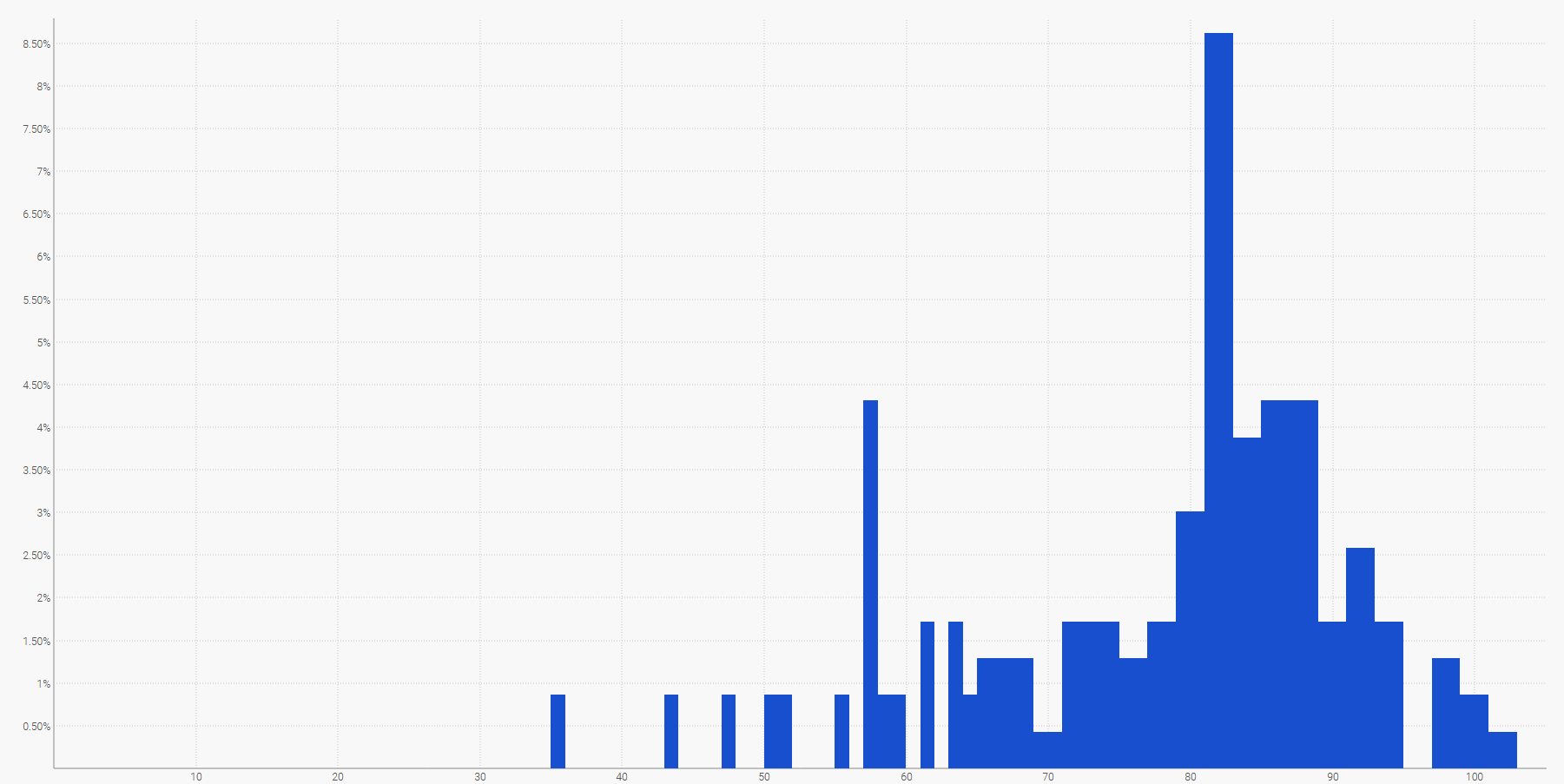
The simplest way to visualize a discrete probability distribution is a histogram, where the vertical axis indicates the probability and the horizontal axis the value of the random variable of interest. For example, a probabilistic forecast of a lead time can be displayed as:


An empirical distribution of the observed lead times in daily buckets.

The future demand, summed over a specified time period, can also be represented by a histogram. More generally, the histogram is well-suited for all the one-dimensional random variables over $\mathbb{Z}$, the set of relative integers.

The visualization of the probabilistic equivalent of an equispaced time-series - i.e. a quantity varying over discrete time periods of equal length - is already much more challenging. Indeed, unlike the one-dimensional random variable, there is no canonical visualization of such a distribution. Beware, the periods cannot be assumed to be independent. Thus, while it is possible to represent a “probabilistic” time-series by lining up a series of histograms - one per period -, this representation would badly misrepresent the way events unfold in a supply chain.


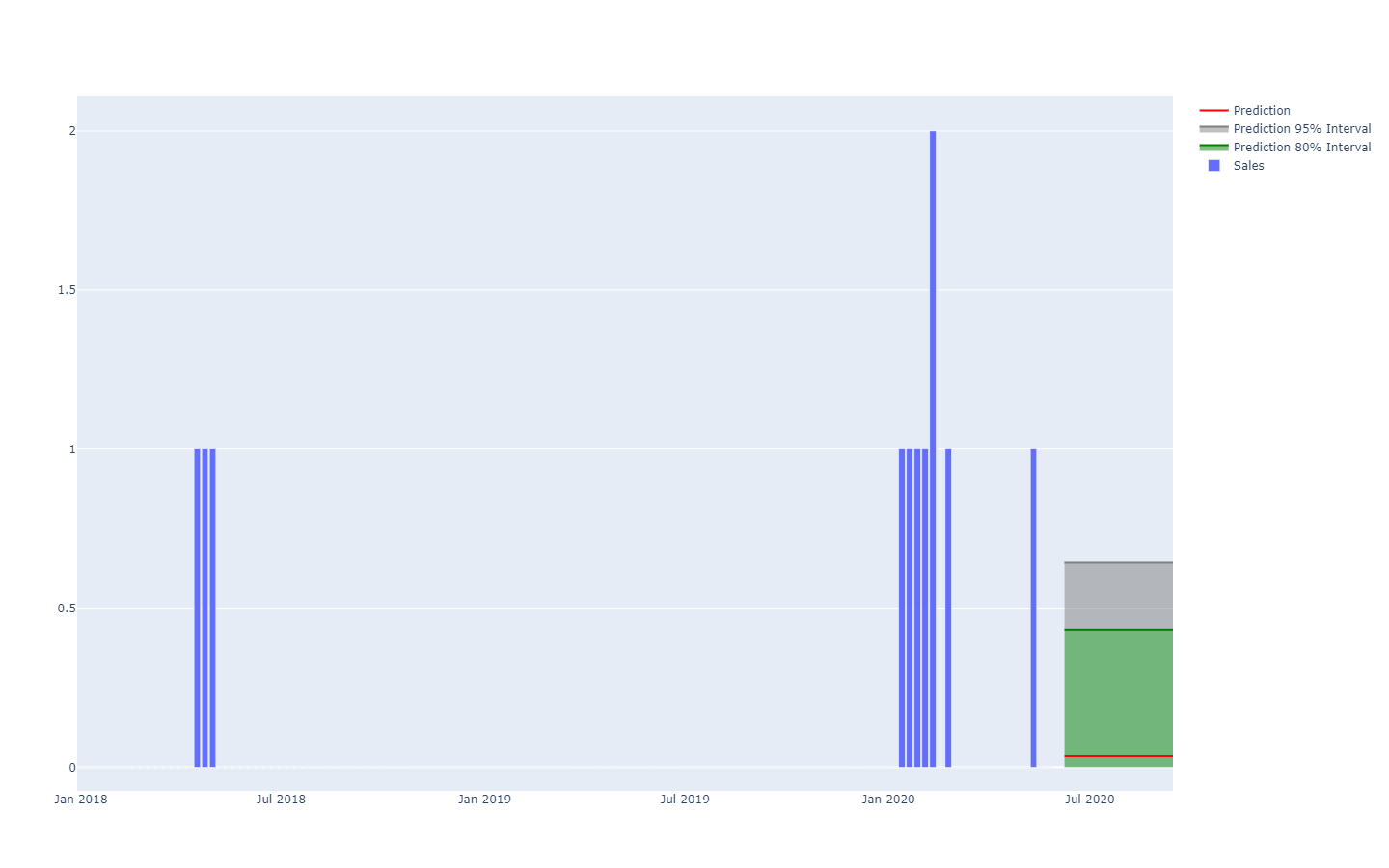
A probabilistic demand forecast represented via quantile thresholds.

For example, it’s not-too-improbable that a newly launched product will perform well, and reach high sales volumes (a hit). It’s not-too-improbable either that the same newly launched product will fail and yield low sales volumes (a miss). However, vast day-to-day oscillations between hit-or-miss sales level are exceedingly unlikely.

Prediction intervals, as commonly found in supply chain literature, are somewhat misleading. They tend to emphasize low-uncertainty situations which are not representative of actual supply chain situations;


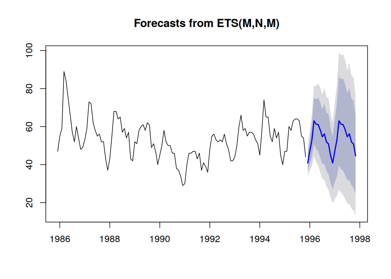
Excerpt from Visualization of probabilistic forecasts, by Rob J Hyndman, 21st November 2014

Notice how these prediction intervals are exactly the probability distributions, put side-by-side with a coloring scheme to outline specific quantile thresholds.

A better representation - i.e. which does not better the strong inter-period dependencies - is to look at the cumulative values over time, taking the quantiles of those, and then differentiate to recover per-period increments (see the first illustration of a probabilistic forecast given at the beginning of the present article). The visualization is the same, but the underlying semantic differs. We are now looking at quantiles over scenarios, outlining the extremely favorable (resp. unfavorable) scenarios.

Probabilistic forecasting antipatterns

Probabilistic forecasts challenge the way many people “intuitively” think about the future. In this section, we cover some of the most frequently misunderstood aspects of probabilistic forecasting.

No such thing as ‘unpredictable’ events

From the deterministic perspective, predicting the outcome of the lottery is impossible, as the odds of getting it right are “one in a million”. However, from a probabilistic perspective, the problem is trivial: every ticket has a “one in a million” chance of winning. The very high variance of the outcome should not be confused with some “unknowability” of the phenomenon itself, which can be perfectly well understood, as is the case for a lottery. Probabilistic forecasting is about quantifying and structuring the variance, not about eliminating the variance.

No such thing as ‘normal’ distributions

Normal distributions, also known as Gaussians, are ubiquitous in both supply chain and physics textbooks. Yet, as far as human affairs are concerned, next to nothing is “normally” distributed. Normal distributions, by design, make large deviations (compared to the average deviations) exceedingly rare, to the point of being ruled-out as plain impossible by the model - i.e. odds lower than one in a billion. Demand, lead time, returns are many patterns that are categorically not normally distributed. The only upside of normal distributions is that they are well-suited to conjure textbook exercises for students, as they lend themselves to explicit analytical solutions.

Cherry-picking probabilities

When confronted with a probability distribution, it is tempting to cherry-pick one point of the distribution, possibly the mean or the median, and proceed based on this number. This process goes against the very essence of the forecast’s probabilistic aspect. Probabilities should not be collapsed into a single point estimate, because no matter which point is chosen, this process incurs a massive loss of information. Thus, while somewhat disturbing, the probabilities are intended to be preserved as such for as long as possible. The point of collapse is typically the final supply chain decision, which maximizes the returns while facing uncertain futures.

Removing statistical outliers

Most classic numerical methods - firmly grounded in the deterministic perspective of the forecasts (e.g. moving averages) - misbehave badly when encountering statistical outliers. Thus, many companies establish processes to manually “clean” the historical data from those outliers. However, this need for such a cleaning process only outlines the deficiencies of those numerical methods. On the contrary, statistical outliers are an essential ingredient of the probabilistic forecast as they contribute to get a better picture of what is happening at the tail of the distribution. In other words, those outliers are the key to quantify the likelihood of encountering further outliers.

Bringing a sword to a gunfight

Specialized tooling is required to manipulate probability distributions. Producing the probabilistic forecast is only one step among many to deliver any actual value for the company. Many supply chain practitioners end up dismissing probabilistic forecasts for a lack of suitable tools to do anything with them. Many enterprise software vendors have joined the bandwagon and now claim to support “probabilistic forecasting” (along with “AI” and the “blockchain”), but never actually went further than cosmetically implementing a few probabilistic models (cf. the section above). Exhibiting a probabilistic forecasting model is worth next to nothing without the extensive tooling to leverage its numerical results.

Notes

[1]: The smooth() function in Envision is handy for regularizing random variables through a discrete sampling process of some kind.

[2]: Prior knowledge about the structure of the problem should not be confused with prior knowledge of the solution itself. The “expert systems” pioneered back in the 1950s as a collection of hand-written rules failed, because human experts fail at literally translating their intuition into numerical rules in practice. Structural priors, as used in differentiable programming, outline the principle, not the fine-print, of the solution.